This post summarizes my experience in building a Structure from Motion (SfM) module in Python. Over the course, this post will go through some of the mathematical underpinnings behind SfM as well as the programming constructs in Python leveraged to accomplish various tasks in the module. You can clone the source code for this tutorial and follow the instructions in the readme to run the code.
Preliminaries
Structure from motion is a technique to perceive depth by utilizing movement. It is based on the human experience of trying to understand the structure of a scene. Imagine a pole lying on the ground some distance away from you in such a way that one of its ends faces your general direction. From your angle and height above the ground, the length of the pole probably looks shorter than it actually is. What do you instinctively do to guage the true length of the pole? You move around it to get a better view of the length. SfM is based on the same principle - that much of the 3D structure of a scene can be determined by 2D snapshots taken at different points in the scene. Bear in mind that the motion can be with respect to an observer in a static scene, or with respect to an object with a static observer. Both cases provide an opportunity to perceive structure, but here, we consider the former.
A camera is represented by a matrix \(P\) which transforms a point \(X\) in the real world to a pixel \(x\) in the image. This relationship is given by the following equation -
$$ x = PX $$
To be able to find X, we need to do the following -
$$ X = P^{-1}x $$
So, finding the camera matrix or the camera pose for each of the images (the 2D snapshots or views) is a part of the process of reconstructing 3D coordinates. SfM, thus, involves estimating the 3D points along with the camera pose from a sequence of images. The 3D points are recovered by a procedure known as triangulation that uses camera poses to accurately locate the points in space.
Incremental and Global SfM
These are two of the prominent pipelines used to solve the SfM problem. Incremental SfM chooses two images as the baseline views, obtains an initial reconstruction, and incrementally adds new images. Global SfM considers all camera poses at once to obtain the reconstruction. My implementation is a simplified version of incremental SfM. Typically, incremental SfM implements some form of view selection or filtering to choose the best image to add to the reconstruction. In this implementation, I use images which have been taken in a sequence and are named in the order in which they have been taken. The baseline views are the first two views in the set, and the subsequent view to be added is the immediately next image in the sequence. This simplifies the implementation significantly, but introduces some errors in the reconstruction which is an acceptable trade-off given that the purpose of this tutorial is to describe the main pipeline behind SfM.
Two-View Geometry
Incremental SfM starts with the two baseline views. In the below figure, two image planes are shown, \(M\) is the point in the 3D world being photographed, \(x\) and \(x’\) are the corresponding image points in each of the views, \(C\) and \(C’\) are the optical centres of the cameras, and \(MCC’\) is the epipolar plane containing the 3D point and the camera centres. \(e\) and \(e’\) are the epipoles, or the images of the camera centers in the opposite views. \(e’x’\) is the image in the second view of the ray passing from \(C\) through \(x\) and is called epipolar line. It is also the line of intersection of the epipolar plane with the second view.
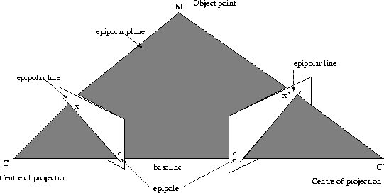
Two-view geometry
The fundamental matrix F
You may be confused by this last piece of information, but what this essentially means is that, for a single 3D point being captured by two views, the point in the second view corresponding to the point in the first view for that 3D point lies along the epipolar line. This is known as the epipolar constraint. If we are trying to find the coordinate in the second view that is looking at the same point as the coordinate in the first view, all we have to do is look across the epipolar line. This geometry is basically encapsulated in a matrix known as the fundamental matrix, which relates a point in one image to a line in another image. The camera matrices can then be obtained from the fundamental matrix, giving us the necessary components required for triangulation (the technique of retrieving the camera matrices from the fundamental matrix is extensively discussed with proof in [1] - Chapter 9).
The essential matrix E
The essential matrix is a representation of the fundamental matrix in the case where we have calibrated cameras. To understand camera calibration and the intrinsic and extrinsic matrix, this is an excellent post that can help you develop the intuition for it. To summarize, a world point is converted to camera coordinates using the extrinsic matrix, which are then converted to homogeneous image coordinates using the intrinsic matrix K. If we apply \( K^{-1} \) to a homogeneous image point \(x\), we end up with something known as the normalized device coordinates (NDCs), which are points transformed into the coordinate system of the camera. Applying the inverse of the extrinsic matrix on NDCs gives us the 3D world coordinates. The NDCs corresponding to a 3D point in a pair of views are related by the essential matrix, similar to how two image points are related by the fundamental matrix.
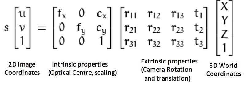
The camera matrix or projection matrix
Now, you may be wondering why any of this matters. This is important because finding the essential and fundamental matrices allows you to decompose them into the extrinsic matrix and ultimately obtain the camera pose or the camera matrix. As mentioned above, the camera pose is a component that is required for triangulation of the 3D points which is what the objective of SfM is. OpenCV, however, does not provide a function to calculate the essential matrix, but we can easily obtain it by calculating the fundamental matrix first (for which there is an OpenCV function) and then derive the essential matrix.
Point Correspondences
Finding the fundamental matrix is done using a variety of techniques, but the 8-point algorithm is a pretty popular approach. Without going too much into the detail of it, the algorithm uses the epipolar constraint to build up a system of homogeneous equations from which the components of the fundamental matrix are computed. For two homogeneous image points \(p\) and \(p’\) in different images looking at the same 3D point, the epipolar constraint is mathematically defined as -
$$ p’^{T}Fp =0 $$
Since the fundamental matrix is defined upto scale, there are 8 unknowns in the matrix to be determined requiring a minimum of 8 point correspondences to solve the system of equations using least squares optimization. Usually, more correspondences are preferred to obtain low errors. In the below system of equations, \(u\) and \(v\) are the x- and y-coordinates of the corresponding points in two different views and \(F_{11} - F_{33}\) are the values of the fundamental matrix.
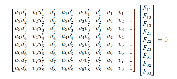
System of equations for the 8-point algorithm
So how do we get 8 or more corresponding points in two images? The solution is to use feature extraction algorithms such as SIFT, SURF and ORB. Since a description of each of these algorithms is beyond the scope of this tutorial, it would suffice to know that these algorithms extract feature points that are considered representative of an image. These feature points are coordinates in the image and are defined by feature descriptors - vectors that uniquely encapsulate certain properties of a point. The idea is that descriptors of two points can be matched using metrics like Euclidean distance to measure how similar they are. Essentially, for a point in one image, we could obtain a list of points in another image that represents the same point in the real world, i.e, we could obtain point correspondences.
View
Each image in the images/ folder is stored in Python as a View data structure. A View object contains essential information about the image such as the image array, image name, list of keypoints and descriptors, and the rotation and translation components of the extrinsic matrix. These last components are calculated gradually for every subsequent View and is used to triangulate new 3D points.
self.name = image_path[image_path.rfind('/') + 1:-4]  # image name without extension
self.image = cv2.imread(image_path)  # numpy array of the image
self.keypoints = []  # list of keypoints obtained from feature extraction
self.descriptors = []  # list of descriptors obtained from feature extraction
self.feature_type = feature_type  # feature extraction method
self.root_path = root_path  # root directory containing the image folder
self.R = np.zeros((3, 3), dtype=float)  # rotation matrix for the view
self.t = np.zeros((3, 1), dtype=float)  # translation vector for the view
Additionally, View also contains functions to read an image from a file on disk, compute features of the specified type, and save the feature information back on disk as .pkl files in a subfolder called features/. Storing the information on disk ensures that we don’t recompute the same stuff over and over again when we are experimenting with the code.
Match
A Match object contains information about the feature matches between any two pairs of images. It contains the indices of the keypoints in each of the images that are similar. The match is performed using the brute-force matcher. For reasons that will be explained later, every view is matched against every other view. Similar to the View class, the Match class also contains functions to compute and store the matches on disk in a subfolder called matches/ to avoid repeated computation.
self.indices1 = []  # indices of the matched keypoints in the first view
self.indices2 = []  # indices of the matched keypoints in the second view
self.distances = []  # distance between the matched keypoints in the first view
self.image_name1 = view1.name  # name of the first view
self.image_name2 = view2.name  # name of the second view
self.root_path = view1.root_path  # root directory containing the image folder
self.inliers1 = []  # list to store the indices of the keypoints from the first view not removed using the fundamental matrix
self.inliers2 = []  # list to store the indices of the keypoints from the second view not removed using the fundamental matrix
self.view1 = view1
self.view2 = view2
Once the features and matches are computed and stored on disk in their respective folders, we begin the main reconstruction loop.
Baseline Pose Estimation
The first two images in the image set are taken as the baseline. What this means is that we consider the position of the first view to be the origin in world coordinates and calculate the position of the remaining views relative to the first pose. The responsibility of kickstarting the reconstruction process lies with the SFM class and it’s reconstruct() function. The class takes a list of Views and a dictionary of Matches and iterates through them to gradually reconstruct the points. The first two views are passed to a Baseline object which specifically estimates the pose for the baseline. The Baseline object does the following steps to compute the pose for the second view -
- Calls the
remove_outliers_using_F()function to calculate the fundamental matrix between the two views. This is done using the OpenCV in-built functionfindFundamentalMat()that uses the 8-point algorithm. Since it is a least squares optimization, we can perform post-processing on the keypoints using the obtained fundamental matrix and remove the points that don’t obey the epipolar constraint. These inliers are stored in the match object and are the final points that are reconstructed. This is easy as the OpenCV function returns amaskarray to filter the points.
mask = mask.astype(bool).flatten()
match_object.inliers1 = np.array(match_object.indices1)[mask]
match_object.inliers2 = np.array(match_object.indices2)[mask]
- Calculates the essential matrix from the fundamental matrix using the following formula -
E = K.T @ F @ K
As mentioned earlier, the essential matrix is a specialization of the fundamental matrix. The proof for the above formula is given in definition 9.6 of Chapter 9 in [1].
- Extracts the rotation and translation elements of the extrinsic matrix from the essential matrix. This procedure is quite lengthy and described in detail in section 9.6.2 of [1]. To summarize, we perform singular value decomposition on the essential matrix ((E\) using the function
get_camera_from_E()and obtain 2 different values each for the rotation and the translation elements - \(R_1\), \(R_2\), \(t_1\) and \(t_2\). This gives us 4 different solutions for the extrinsic matrix based on the number of combinations possible. These four solutions are subsequently checked for their validity in thecheck_pose()function and the correct pair is chosen as the extrinsic matrix of the second view. For more information, check the comments for the functions in thebaseline.pyfile and Chapter 9 in [1].
Triangulation
Now that we have computed poses for two views, the next step is triangulation. Triangulation is the process of using 2D image points as well as pose information to reconstruct 3D points. Applying the inverse of the camera matrix on an image point gives us a ray passing through the point. After acquiring the ray of the corresponding point in the second view, we can find the the 3D point by finding the point of intersection of the two rays. This is the basic theory behind triangulation.
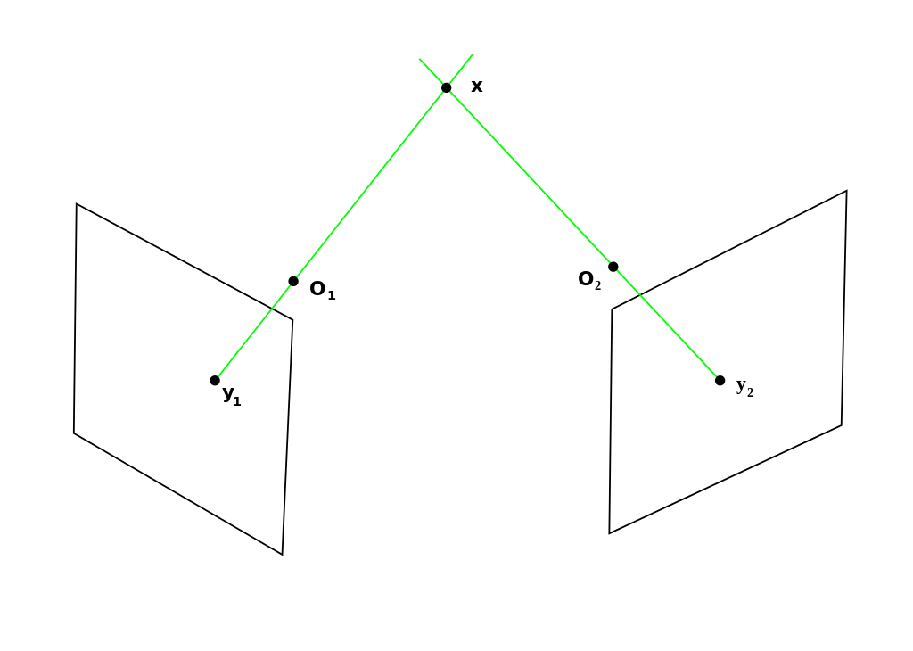
Triangulation.
The function triangulate() loops through the inlier points from two views and calls the get_3D_point() function to obtain the 3D point. The triangulation method used in get_3D_point() is provided in Chapter 4 of [2], but alternately, we can also use the OpenCV function triangulatePoints() for the same purpose. Note that while the function in my code operates on a point-by-point basis, the OpenCV function takes a set of points.
Reprojection error
The reprojection error is an accuracy metric for reconstruction problems. For each triangulated point, we project the 3D point back on the image plane using the camera matrix and compare the result with the 2D point that was used in the triangulation. Since triangulation is a least squares optimization problem, it has an error term involved. Calculating the mean reprojection error everytime we intergrate a new view gives us an idea about how off the triangulation is and allows us to apply a technique called bundle adjustment to minimize the error. Bundle adjustment is not implemented in the code, but it would suffice to know that the technique uses the reprojection error as an objective to minimize and makes corrections to the computed camera poses as well as the triangulated points. The following snippet is from the function that calculates the reprojection error for a point -
reprojected_point = K.dot(R.dot(point_3D) + t)
reprojected_point = cv2.convertPointsFromHomogeneous(reprojected_point.T)[:, 0, :].T
error = np.linalg.norm(point_2D.reshape((2, 1)) - reprojected_point)
The triangulated points are stored in self.points_3D and are now ready to be plotted. For plotting, I use Open3D, which converts my Numpy array of 3D points into a data structure that can be written into a .ply file. The .ply files are written inside the points/ subfolder. Let’s visualize some of the results.

Image from fountain-11 folder of the OpenMVG benchmark
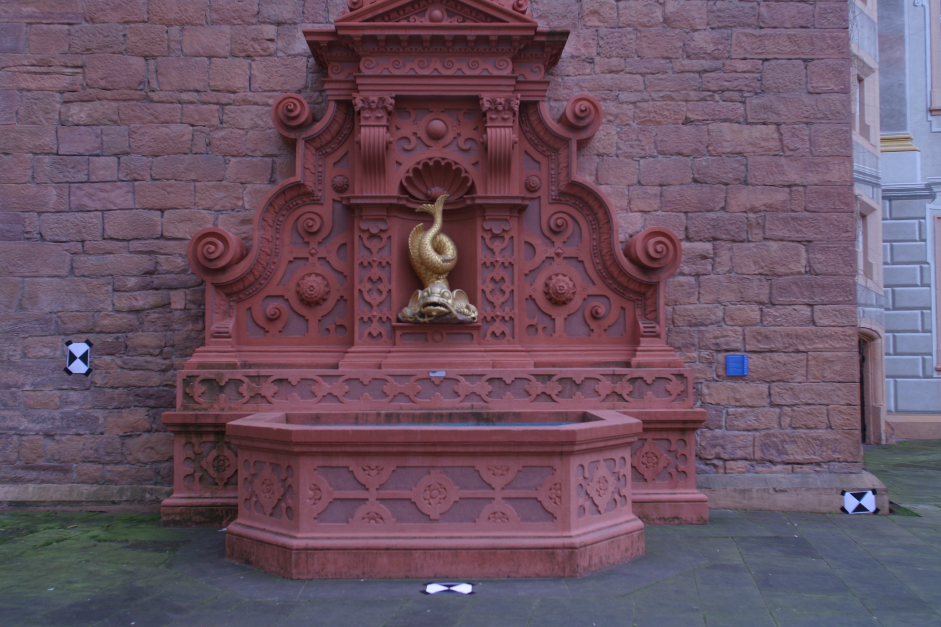
Image from fountain-11 folder of the OpenMVG benchmark

Image from fountain-11 folder of the OpenMVG benchmark
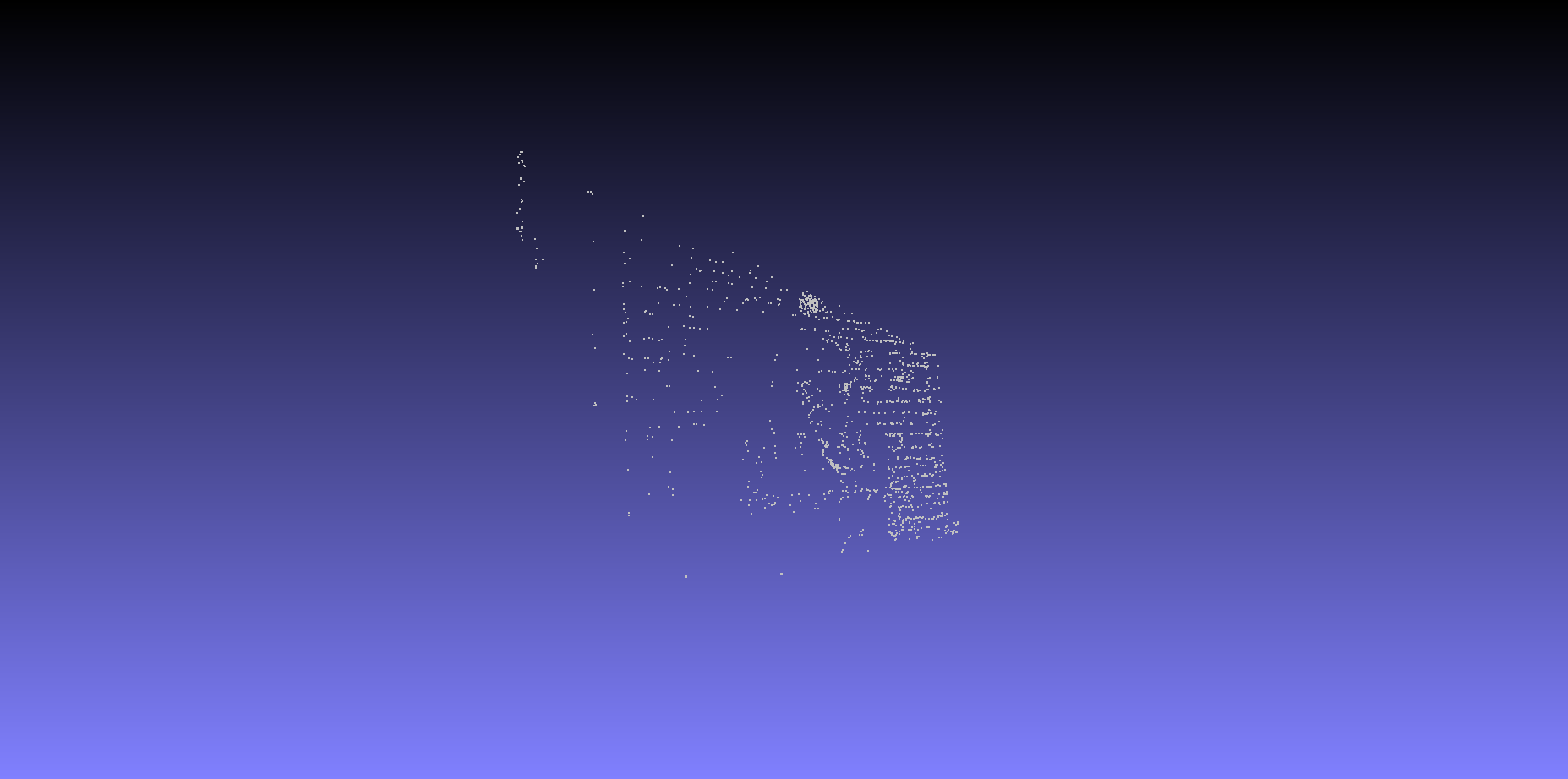
Triangulation result from baseline
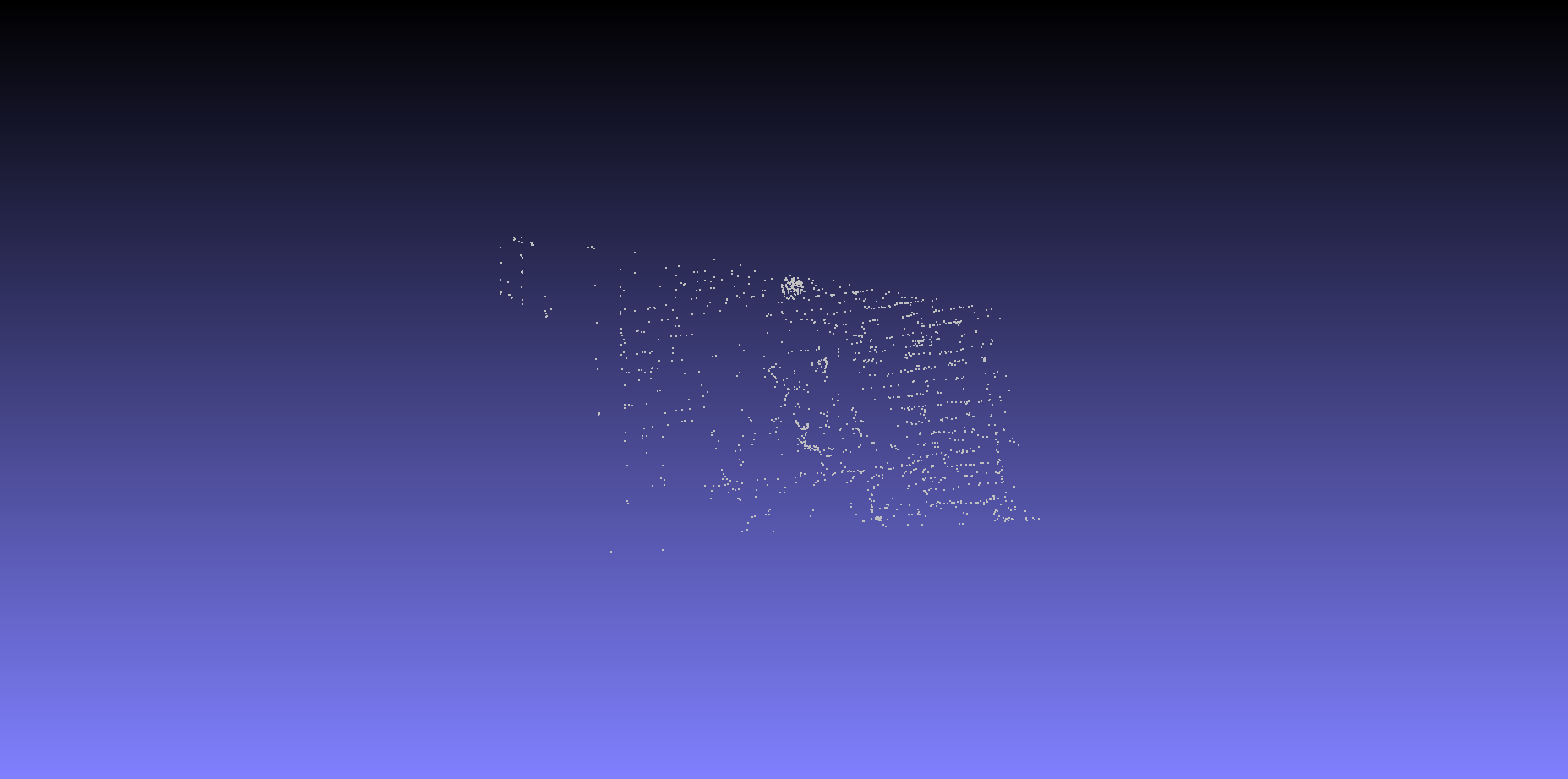
Triangulation result from baseline
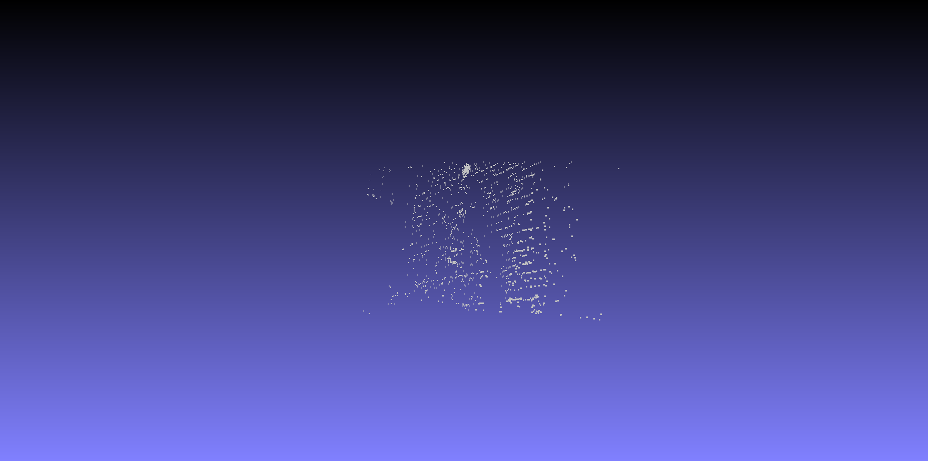
Triangulation result from baseline
Integrate New View
Ideally, the next view to be added to the reconstruction would be filtered and chosen using some criteria, such as number of keypoints and matches. But since we are processing all images sequentially, the next view to be added is simply the next image taken in order of the naming.
To compute the pose of the new view, we use a technique called Perspective n Point. The technique uses components of the new view such as 2D points, the intrinsic matrix, and the 3D points to compute it’s pose. But, wait, we don’t have the 3D points from the new view. What we can do, instead, is make use of the 3D points triangulated in the previous steps whose corresponding image points have matches in the new view. This requires quite a bit of bookkeeping. As a result, we store a record of all the 3D points triangulated in a dictionary called self.points_map where the key is a tuple of (view_index, index_of_keypoint_in_the_view) and the value is the index of the 3D point in self.points_3D. Given an old keypoint, we can extract, if any, the 3D point it contributed to. This is done immediately after triangulation of a point.
self.point_map[(self.get_index_of_view(view1), match_object.inliers1[i])] = self.point_counter
self.point_map[(self.get_index_of_view(view2), match_object.inliers2[i])] = self.point_counter
self.point_counter += 1
Thus, we extract the keypoints in the new view which has a match against a keypoint in an older view that was triangulated. This gives a list of image points in the new view and a list of 3D points that they possibly point to (through their matches). This is the input to the solvePnPRansac() function which estimates the pose of the new view. RANSAC is used to filter outliers. Now that we have obtained the pose for the new view, we go through the matches of the new view with all of the old views to triangulate points that have so far not been triangulated. The matches information was computed in one of the initial step for every view with every other view, and now the reason for that is apparent.
Conclusion
Some of the images might not yield accurate reconstructions because of the lack of bundle adjustment. Incremental SfM is a gradual process of refining the reconstruction of a scene. Errors made in estimation in the previous steps can easily propagate to later steps and contribute to a reprojection mismatch. However, what is important here is the pipeline followed to obtain a reconstruction. To reiterate, we start with two baseline views, the second of which we compute the pose for, after which we triangulate 3D points between them. We then incrementally add new views by first computing their pose using Perspective n Point and then triangulating new points in the scene.
References
- Hartley and Zisserman’s Multiple View Geometry in Computer Vision
- Packt’s Mastering OpenCV with Practical Computer Vision Projects